liste

Bonjour et bienvenue dans mon site ! Willkommen auf meiner Seite! welcome in my homepage! http://assistance-en-sig.blogspot.com/ SIG ; Bases de données ; Géomatique; Python; ArcGIS; QGIS;

recherche

Showing posts with label arcgis 10. Show all posts

Wednesday, August 21, 2013

Extend Crime Analysis with ArcGIS 10 Spatial Statistics Tools

By Lauren Scott and Nathan Warmerdam

Editor's note: Crime mapping using traditional GIS analysis techniques has been helping law enforcement agencies track crime incidents and produce density maps showing overall crime patterns. With improvements in the availability and quality of crime data in digital format and more robust GIS software, police departments have expanded the use of GIS. They are using spatial data analysis to assess crime patterns, optimize resource allocation, and improve emergency call response. The spatial statistics tools in ArcGIS enhance spatial data analysis of crime data by supplying tools that use statistical methods designed specifically for use with spatial data. This article describes how the Hot Spot Analysis, Mean Center, Linear Directional Mean, and Standard Deviational Ellipse tools, available at all license levels, can be used for more sophisticated types of crime analysis.

Understanding Where Crime Occurs

Crime hot spots are areas of high crime intensity. Knowing where crime is concentrated helps law enforcement agencies make better decisions about allocating police resources. In addition, using GIS to map crime hot spots can effectively communicate crime patterns and crime prevention strategies to decision makers and the public.
The Hot Spot Analysis tool in ArcGIS 9 identifies spatial clusters of statistically significant high or low attribute values. Given a set of weighted data points, such as the number of crimes per census block, and operating under the expectation that data values are randomly distributed across the study area, this tool delineates clusters of census blocks with higher than expected crime incidents. These clusters are hot spots. The Hot Spot Analysis tool also delineates spatial clusters of lower than expected crime incidents. These clusters reflect crime cold spots and may provide clues about policy or environmental factors that discourage crime.
click to enlargeclick to enlarge
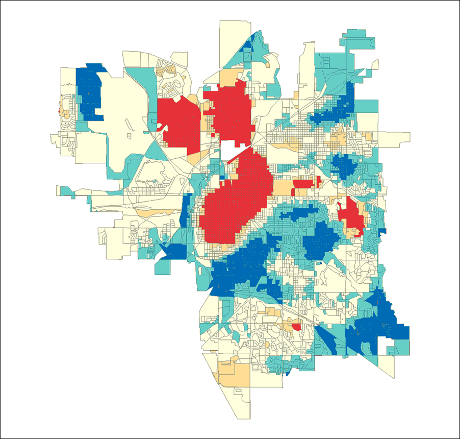
Crime hot spots generated from vandalism data for Lincoln, Nebraska, that have not been normalized. Hot spots are shown in bright red and located in downtown Lincoln, an area with a large population. Cold spots, or areas of low crime, are shown in dark blue and are located in suburban areas.Hot spot analysis using vandalism data that was normalized with data from all crime incidents for Lincoln, Nebraska. Again, areas with high incidence of vandalism are shown in bright red and low vandalism areas are shown in dark blue.
Running the Hot Spot Analysis tool against raw total crime counts provides the analyst with an overall picture of crime patterns. A map of these crime patterns effectively communicates where crime activities are highest and where they are lowest. However, the police officers working in the study area day to day will likely already know firsthand where crime activities are highest. Often more useful are analyses that incorporate risk assessment by controlling study area variations in population, overall crime patterns, and environmental factors.

Performing Risk Assessment

One would expect more crimes in areas with more people and fewer crimes in areas with fewer people. Communities are a tapestry of neighborhoods (each one with different characteristics). In essence, a study area can be viewed as a landscape of crime. Gang activities; the types of businesses in an area; and factors that can be difficult to quantify, such as lighting, access to freeways, or a high proportion of residents with criminal records, can drive up the crime rate in some neighborhoods.
For example, if the task is to determine where to implement a vandalism prevention program, simply running the Hot Spot Analysis tool on raw vandalism counts will probably find hot spots just where they would be expected (in downtown areas that have lots of people and, typically, lots of crime). However, dividing vandalism counts in each census tract by all crime counts will represent vandalism counts as a proportion of all crime events. Running the hot spot analysis on these normalized ratios will provide a different picture. It will show the location of clusters of tracts in which vandalism represents a larger than expected proportion of all crime events. Such an analysis, carried out on crime data from Lincoln, Nebraska, showed that vandalism is primarily a suburban issue. Consequently, implementing a vandalism prevention program in the downtown area probably would not be as effective as implementing a program in the suburbs where vandalism constitutes a larger proportion of overall crime events.
click to enlargeclick to enlarge
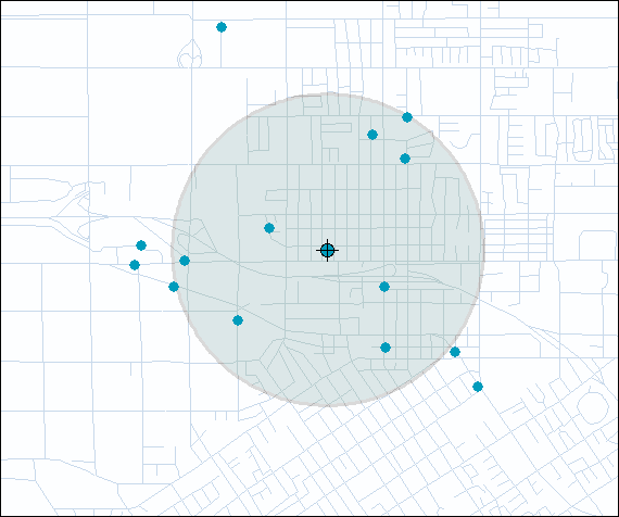
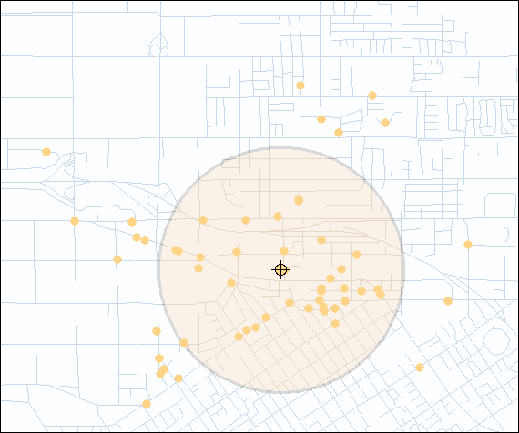
Daytime burglaries tend to be slightly more concentrated than nighttime burglaries, indicated by the smaller standard distance circle. These circles also highlight the differences in the locations of daytime and nighttime burglaries.

Looking for Clues to Criminal Activities

One of the simplest approaches to better understand some factors that encourage criminal activity is examining the distribution of different types of crimes. A crime analyst, for example, might want to know if the mean center for burglaries shifts when evaluating daytime versus nighttime crime incidents. This information could be used to improve the way police departments assign personnel. The Mean Center tool available in ArcGIS 9 computes the average x-coordinate and y-coordinate for each crime incident in the study area.
Another new tool for studying the distribution of crime incidents works with line data. The Linear Directional Mean tool is used to measure the trend of either the direction or orientation of line features by calculating the average angle of the lines. This statistic can be used to evaluate auto theft data that contains information on the location from which each vehicle was taken and where it was eventually recovered. Analyzing this data using the Linear Directional Mean tool highlights recurring patterns that can suggest an underlying infrastructure supporting car thefts in the region. Similar analysis has been used to study data on missing/abducted children.
click to enlarge
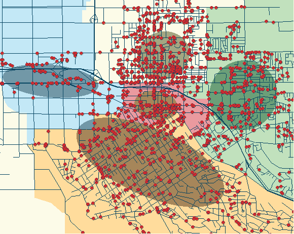
Analysis of the spatial dispersion of crimes by police beat in Redlands, California, shows that crimes in the western portion of the city follow major transportation networks in the area.
When crime distributions are compared to other features in the landscape, similarities or relationships often become apparent. The most common way for measuring the trend for points or areas is to calculate the standard distance separately in the x and y directions. These two measures define the axes of an ellipse encompassing the distribution of features. The ellipse is referred to as the standard deviational ellipse since the method calculates the standard deviation of the x-coordinates and y-coordinates from the mean center to define the axes of the ellipse. This ellipse shows if the distribution of features is elongated, which indicates it has a particular orientation.
For example, crime events grouped by police beat and evaluated using the Standard Deviational Ellipse tool may show that, for some police beats, crime activities are evenly distributed throughout the beat so the ellipse resembles a circle. In other cases, crime activities tend to follow road networks, and crime incidents in these police beats show that orientation.

Conclusion

By placing crime incidents in a geographic context and applying the spatial statistical analysis tools now available in ArcGIS 9, crime analysts can better understand where and why crime activity is occurring and law enforcement agencies can respond in the most efficient and effective manner.

Additional Resources

Not only crime analysts but also GIS practitioners in many research areas, such as epidemiology, archaeology, wildlife biology, and retail analysis, will benefit from the spatial statistics tools in ArcGIS 9. These tools can be easily modified or extended because most were written using the Python scripting language. The source code for the statistical tools can be accessed from ArcToolbox and serve as samples and templates for further customization. For more information about scripting in the ArcGIS geoprocessing environment, select Geoprocessing >Writing Geoprocessing Scripts on the Contents tab of the ArcGIS 9 Online Help.
click to enlarge
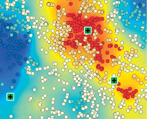
Analysis of 911 emergency calls shows regions that get many calls in bright red and regions that get few calls in dark blue and the relationship of those areas to local police and fire response stations, indicated by bright green squares.
The Esri Guide to GIS Analysis, Volume 2, an Esri Press book scheduled for release in the third quarter of 2005, provides additional specific information on spatial statistics tools and more general information on spatial data analysis using GIS. It is the second in a series by Andy Mitchell. The first book,The Esri Guide to GIS Analysis, Volume 1, focuses on visual and cartographic methods of spatial data analysis. Both books can be purchased online at www.esri.com/shop.
Online resources are also available. A five-minute video showing hot spot analysis of emergency 911 call data is available on the Esri Web site. An article describing the tools in the Spatial Statistics toolbox appeared in the October–December 2004 issue of ArcUser and is available online. For more information on the Python scripting language, visit www.Python.org.

About the Authors

Dr. Lauren Scott works on the ArcGIS Geoprocessing Team and developed the tools in the Spatial Statistics toolbox. She holds a Ph.D. in geography from the joint doctoral program at San Diego State University in California and the University of California, Santa Barbara.
Nathan Warmerdam works as a product specialist on the Geoprocessing Team. He holds a master's degree in geographic information science from the University of Redlands in California.
source esri.com

Tuesday, August 20, 2013

Procédure d'installation d'ArcGIS DeskTop 9.3 (Désinstallation ArcGIS DeskTop 9.2)

Résumé
Cet article technique vous permettra de désinstaller votre ArcGIS DeskTop 9.2 afin de pouvoir installer la version 9.3 d'ArcGIS Desktop.


Description
 Cet article contient des instructions modifiant certains paramètres du système d'exploitation. Une modification non conforme de ces paramètres peut engendrer de sérieux problèmes. Esri recommande au préalable de réaliser une sauvegarde complète du système d'exploitation, et particulièrement de la base de registre, avant de mettre en application les solutions proposées. Esri ne peut garantir la résolution du problème résultant d'une utilisation incorrecte de l'éditeur de la base de registre.

Partie I – Désinstallation de la Francisation d’ArcGIS DeskTop et des outils complémentaires non supportés.
   1. Désinstaller tous les outils complémentaires non supportés :


   Pour les utilisateurs ayant installé des outils complémentaires non supportés depuis le site du support d’Esri France ou d'autres sites Internet, il est fortement conseillé de suivre cette première étape de la désinstallation.

   Pour les utilisateurs n’ayant jamais installé d’outils complémentaires non supportés, vous pouvez passer directement au point 2.

         1.1. Procédure de désinstallation des dll liées aux outils complémentaires non supportés :
         Aller dans le menu démarrer de Windows puis Exécuter. Saisir la commande :

         regsvr32 -u "C:\Temp\LegendeBivariee.dll"
 (en tapant votre chemin d'accès complet où est stockée la *.dll à la place de C:\Temp\LegendeBivariee.dll) puis faites Ok.

         Recommencer la commande regsvr32 -u pour chaque outil complémentaire non supporté présent sur votre poste.

         Si vous vous ne souvenez plus où sont stockées les *.dll, vous pouvez retrouver leurs chemins d'accès dans la base de registre, comme indiqué ci-dessous.

         Procédure pour identifier le chemin d'accès aux dll :

         Faire Menu Démarrer de Windows et taper REGEDIT, puis aller dans le dossierHKEY_CURRENT_USER\Software\Microsoft\Windows\CurrentVersion\Explorer\ComDlg32\OpenSaveMRU\dllpour obtenir le chemin d’accès à la DLL (copier le chemin d’accès pour le réutiliser avec la commande regsvr32 –u.
         D’autres outils non supportés téléchargés sur Internet peuvent également être présents sur votre ordinateur sous forme de .exe ou .bat (par exemple : Hawths Analysis Tools). Vous devez utiliser pour ces outils le fichier Uninstall livré avec l'outil pour les désinstaller.

         1.2. Désinstaller le service pack (SP) Français pour ArcGIS DeskTop (Panneau de configuration -> Ajout-Suppression de programmes).

         1.3. Désinstaller ArcGIS DeskTop version Française (Panneau de configuration -> Ajout-Suppression de Programmes).

Partie II – Désinstallation de la version Anglaise
Deux possibilités sont envisageables à ce niveau :

Première possibilité : Utiliser l’utilitaire 93ConflictDetector.exe afin de désinstaller l’ensemble des produits ArcGIS version finale et Anglaise.Voici le lien pour télécharger cet utilitaire :
http://support.Esri.com/index.cfm?fa=downloads.samplesUtilities.viewSample&PID=17&MetaID=1414

Deuxième possibilité : Faire la désinstallation manuelle de l’ensemble des produits ArcGIS version finale et Anglaise.
Il s’agit de désinstaller :

         2.1. Désinstaller Tutorial Data (Panneau de configuration -> Ajout-Suppression de programmes, s'il est installé).

         2.2 . Désinstaller Developper kit (Panneau de configuration -> Ajout-Suppression de programmes, s'il est installé).

         2.3. Désinstaller Crystal report 
(Panneau de configuration -> Ajout-Suppression de programmes, s'il est installé).

         2.4. Désinstaller ArcGIS Desktop
.


Partie III – Désinstallation de Python
A partir du Panneau de configuration -> Ajout Suppression de programmes, désinstaller Python 2.4.1 et les autres logiciels installés liés à Python 2.4.1. (s’il y en a, comme par exemple Python combined).

Partie IV – Suppression des dossiers Esri d'ArcGIS Desktop 9.2
         4.1. Tout d’abord, renommer le dossier Esri en Esri_OLD pour les emplacements suivant :
         C:\Documents and Settings\VotreProfilUtilisateur\Application Data\Esri et C:\Program Files\Fichiers communs.

         4.2.
 Ensuite, renommer également les dossiers Esri se trouvant dans la base de registre.

         Pour cela, naviguer dans le menu Démarrer de Windows -> Exécuter -> puis saisir regedit et faire Ok .

         Naviguer vers le dossier HKEY_CURRENT_USER/Software/Esri et renommer le en Esri_OLD

         Naviguer vers le dossier HKEY_LOCAL_MACHINE/Software/Esri et renommer le en Esri_OLD

         4.3.
 Ensuite, sur votre disque dur, veuillez supprimer le dossier ArcGIS et Esri sur votre C:\Program Files.

Partie V – Nettoyer le registre de Windows
         Pour terminer, il est souhaitable de nettoyer votre base de registre en utilisant un outil de nettoyage de registre tel que RegCleaner ou CCleaner. Il vous permettra de supprimer toutes les clés liées à Esri, ArcGIS et outils liés (Python).

          Les problèmes liés à l'installation ou à l'utilisation de ces utilitaires ne peuvent en aucun cas être pris en charge par le support technique d'Esri France, ces derniers doivent être utilisés avec grande précaution car si vous supprimez par inadvertance une clef de registre liée au système ou à un autre logiciel des dysfonctionnements importants peuvent apparaître.
Partie VI – Installation d’ArcGIS Desktop 9.3
         6.1. Il ne vous reste plus qu’à effectuer l’installation d’ArcGIS 9.3 à partir du DVD d'installation.

         6.2.
 Après l’installation d’ArcGIS 9.3, il est recommandé d’effectuer un Réparer d’ArcGIS. Il s’agit de retrouver les fonctionnalités liées à l’éditeur Visual Basic (Article technique Esri Inc pour plus d'informations : Lien. Pour ce faire, aller dans le Panneau de configuration -> Ajout ->Suppression de programmes et pour ArcGIS Desktop faites modifier. Dans la fenêtre suivante, cliquez sur Réparer.

         6.3.
 Vous pouvez ensuite enregistrer votre licence (code UNK + 9 chiffres) à la fin de l’installation afin d’activer ArcGIS Desktop. Si cette étape ne fonctionne pas, veuillez vous rendre sur le site https://service.Esri.com/ et vous placer sur l’onglet « Product Registration ». Veuillez suivre les étapes et soumettre votre demande d’enregistrement de licence. Vous recevrez par mail le fichier de licences. Attention, ce mail peut parfois être considéré comme Spam dans votre messagerie.

         6.4.
 Pour terminer, vous pouvez installer le supplément français ArcGIS 9.3 (CD version française) .

Saturday, May 25, 2013

TELECHARGER ArcGis 10 Crack with EASY TutoriaL

Image 


Salut, Voici un guide simple à installer et le crack ArcGIS 10! Suivez ce guide étape par étape et tout devrait fonctionner parfaitement! Je n'ai pas inventé les fichiers dernières, enfin, je viens de constater que beaucoup de peuples où la difficulté à se fissurer ArcGIS et a décidé d'aider ... C'est pour tester le seul programme! Si vous prévoyez de faire de l'argent avec elle, alors, il Achetez! Dans ce tutoriel, j'utilise souvent le "Program Files (x86)" C'est parce que la destination que je suis sur un système 64 bits! Vous pouvez avoir un système 32 bits, puis le vôtre sera "Program Files" ... Désolé pour mon mauvais anglais écrit Nous avons d'abord besoin d'installer le gestionnaire de licences (Non ArcGis programme principal encore!)01 - Télécharger ArcGIS 10 de ce forum (ne se soucient pas de la fissure à venir avec elle!) 02 - Ouvrez le dossier ArcGIS et accédez à "Desktop / Licence» et commencer à "Setup.exe" 03 - Lorsque l'installateur fenêtres ouvertes cliquez sur "Suivant, J'accepte, Suivant, Suivant, Suivant", puis laisser s'installer ... Puis "Terminer" 04 - Après l'installateur a terminé, une fenêtre ouverte! Cliquez sur «Annuler»


 TELECHARGER 

http://www.mediafire.com/file/0w637taxcwin80u/Crack_in_the_wall.zip

http://www.filesonic.com/file/1490123974/Crack_in_the_wall.zip

Saturday, May 11, 2013

Wednesday, May 8, 2013

New: Keygen for ArcGIS 10.1 download for free

Use the links below to download the crack for arcgis 10.1 for free without registration.


Download
Télécharger
Runterladen

If you are satisfied thanks for making a donation by clicking one of the ad.

Saturday, April 27, 2013

TELECHARGER ArcGis 10 Crack with EASY TutoriaL

Image 


Salut, Voici un guide simple à installer et le crack ArcGIS 10! Suivez ce guide étape par étape et tout devrait fonctionner parfaitement! Je n'ai pas inventé les fichiers dernières, enfin, je viens de constater que beaucoup de peuples où la difficulté à se fissurer ArcGIS et a décidé d'aider ... C'est pour tester le seul programme! Si vous prévoyez de faire de l'argent avec elle, alors, il Achetez! Dans ce tutoriel, j'utilise souvent le "Program Files (x86)" C'est parce que la destination que je suis sur un système 64 bits! Vous pouvez avoir un système 32 bits, puis le vôtre sera "Program Files" ... Désolé pour mon mauvais anglais écrit Nous avons d'abord besoin d'installer le gestionnaire de licences (Non ArcGis programme principal encore!)01 - Télécharger ArcGIS 10 de ce forum (ne se soucient pas de la fissure à venir avec elle!) 02 - Ouvrez le dossier ArcGIS et accédez à "Desktop / Licence» et commencer à "Setup.exe" 03 - Lorsque l'installateur fenêtres ouvertes cliquez sur "Suivant, J'accepte, Suivant, Suivant, Suivant", puis laisser s'installer ... Puis "Terminer" 04 - Après l'installateur a terminé, une fenêtre ouverte! Cliquez sur «Annuler»


 TELECHARGER 

http://www.mediafire.com/file/0w637taxcwin80u/Crack_in_the_wall.zip

http://www.filesonic.com/file/1490123974/Crack_in_the_wall.zip

Tuesday, April 23, 2013

XTools Pro - Extension for ArcGIS

XTools Pro is a comprehensive set of useful vector spatial analysis, shape conversion, and table management tools for ArcGIS that greatly enhances ArcGIS functionality and allows ArcGIS users to get to a new level of efficiency and performance. 

XTools Pro includes more than 60 tools for vector spatial analysis, shape conversion, and table management and 40 geoprocessing tools. The most essential functions are collected in a single toolbar for ArcGIS users. New useful tools help save your time and open up unique opportunities for working with geographical data.

Latest version - XTools Pro 9.2

  • Export Table to MS Excel
    - The tool has been completely redesigned with .NET in order to improve stability, performance and usability
    - Name changed to Export Table to MS Excel
    - New unified user interface in all three tools for exporting tables
    - Provides better exporting performance, especially when exporting larger tables
    - Supports larger datasets/tables for exporting (size limit still depends on the available memory)
    - Now you can see not only field names but also field aliases and types
    - Fields in the list can be sorted by name, alias or even type, in either ascending or descending order
    - Fields are now selected using checkboxes which allows for more robust selections (now you won’t lose the selection by accident with a wrong mouse click)
    - Added buttons to fast select/unselect all fields and invert current selection
    - Now you can optionally export descriptions for coded values and subtypes instead of codes
    - Now you can optionally open exported Excel Workbook files after exporting
  • Export Table to TEXT
    - The tool has been completely redesigned with .NET in order to improve stability, performance and usability
    - New unified user interface in all three tools for exporting tables
    - Now you can see not only field names but also field aliases and types
    - Fields in the list can be sorted by name, alias or even type, in either ascending or descending order
    - Fields are now selected using checkboxes which allows for more robust selections (now you won’t lose the selection by accident with a wrong mouse click)
    - Added buttons to fast select/unselect all fields and invert current selection
    - Now you can optionally export descriptions for coded values and subtypes instead of codes
    - Now you can optionally open exported text files after exporting
  • Export Table to HTML
    - New unified user interface in all three tools for exporting tables
    - Now you can see not only field names but also field aliases and types
    - Fields in the list can be sorted by name, alias or even type, in either ascending or descending order
    - Fields are now selected using checkboxes which allows for more robust selections (now you won’t lose the selection by accident with a wrong mouse click)
    - Added buttons to fast select/unselect all fields and invert current selection
    - Now you can optionally export descriptions for coded values and subtypes instead of codes
  • Create Fishnet
    - The tool has been redesigned from scratch with .NET in order to extend functionality and improve usability making Create Fishnet one the most advanced tools for creating fishnets in ArcGIS. In addition to fishnets of rectangular cells it is now possible to build hexagonal cells.
  • Export Data to KML
    - Layers with features classified by value ranges (e.g. graduated colors) now can be correctly exported to KML (KMZ) files
  • Identify Pro
    - Improved performance, especially when identifying numerous features from many layers
    - Added status bar that shows number of identified features and a progress bar
    - Default identified layer set back to "Top-most layer"
    - Other improvements in functionality and stability fixes
  • Other changes
    - New 14-days trial period
    - Other minor bug fixes and enhancements


Current version: XTools Pro 9.2
Zip file size: 63 Mb

Requirements:

Disk space: 69 Mb
Operating system: 
Microsoft Windows 2000/XP/Vista/7
Requisite software: 
ArcGIS desktop 9.2, 9.3, 9.3.1, 10 and 10.1


Saturday, March 30, 2013

New: Keygen for ArcGIS 10.1 download for free

Use the links to download the crack for arcgis 10.1 for free without registration


Download
Télécharger
Runterladen

If you are satisfied please make a donation by clicking one of the ads Thanks
Si vous trouvez ce lien utile merci de faire un don en cliquant sur l'un des liens publicitaires dans le cadre

Monday, March 18, 2013

arcgis 10 crack for windows 8 64 bits rapidshare download

Microsoft has recently released Windows 8 and we have just released ArcGIS 10.1 Service Pack 1.  I’m pleased to announce that Windows 8 and Windows Server 2012 are now supported operating systems for ArcGIS 10.1 SP1.

download here

source rapidshare dot com

Thursday, January 31, 2013

New: ArcGIS 10 tutorials


This page provides a set of various ArcGIS tutorials used to perform a number of common tasks in ArcGIS. Find the tutorial that you would like to work through by clicking the links below. These are Esri tutorials
To work through the ArcGIS Desktop tutorials, you need to install the tutorial data from the ArcGIS Desktop Tutorial Data setup, which is part of the ArcGIS Desktop installation download or media. If the tutorial data has been installed on your system, look for it in C:\arcgis\ArcTutor (the default installation location). In many cases, you will need write access to that location to perform the tutorial.
The ArcGIS Server Installation does not include tutorial data. Most of the ArcGIS Server tutorials are written in a generic way so that you can follow the steps using your own datasets.
These tutorials are published by ESRI:

Database servers:

This tutorial shows you how to use ArcGIS Desktop to use database servers (instances of SQL Server Express) and the geodatabases you create on the database servers to store, access, and edit GIS data. An ArcEditor or ArcInfo license is required to complete the tutorial.
Editing:
In this tutorial, you'll learn the basics of the editing environment in ArcMap, including creating new features on the map; updating attribute values; utilizing snapping while editing, creating, and editing annotation; using topology to maintain spatial integrity; and performing spatial adjustments on your data.

Geodatabases
In this tutorial, you'll learn to build geodatabases that include relationship classes, subtypes, attribute domains, topology, geometric networks, and feature-linked annotation. An ArcEditor or ArcInfo license is required to complete the tutorial.


Sunday, December 16, 2012

Introduction to ArcGIS 10 exercise


Introduction to ArcGIS 10 exercise 


2011 Charlie Schweik


Note: This work is licensed under the Creative Commons AttributionNonCommercial-ShareAlike 3.0 Unported License. To view a copy of this 
license, visit http://creativecommons.org/licenses/by-nc-sa/3.0/. 

This exercise is designed to help you get familiar with elements of ArcGIS – specifically
ArcMap and the “Catalog” window (also called “ArcCatalog”).

Note: Data for all exercises are available at:  
http://courses.umass.edu/nrc592g-cschweik/data.html

Lab Setup
1. Get data files
a. The data we will use is available on the course calendar under today's date. It
is a zip file. Create a folder on your C: drive called “C:/temp/gisdata”. Click
on the link under today's class entry on the course calendar and save to
c:/temp/gisdata (unless I tell you otherwise in class).
b. Using My Computer, navigate to c:/temp/gisdata. Right-click and unzip the
introArcGISdata.zip (use unzip to here). You should see the following files
appear:
• cut_tm_reg_chitwan_00.rrd (satellite image file of an area of Nepal)
• cut_tm_reg_chitwan_00.img (satellite image file of an area of Nepal)
• fmisheadworks.mdb (geodatabase file of irrigation headwork points)
• headworkcov, info folders (arc info coverage)
• a bunch of files with the first name “hw”. One has an extension of
.shp (ArcView shape file).
Getting Started: Let’s look at the Menus of ArcMap
1. Start up ArcMap 10 (Start, programs, ArcGIS, ArcMap 10).
 Create a new “blank map.” Click “OK” on the ArcMap – Getting Started page.
 An untitled, ArcMap document should appear.

Note the “Table Of Contents” section on the left side of the screen.
There are the Magnifier and other tools in one of the icon rows below the main
menus.  2
The main “map area” is the large area below the menu and icon bars that covers
the middle and the right side of the screen.
Look at the main menu. It follows the general standard kind of menu system
File – Add layers, print functions, open or new ArcMap, save, page
properties, etc.
Edit – copy, cut, paste, paste special, find
Bookmarks – this menu allows you to create and manage particular
geographic locations that you can save and reference later. This might be a
study region, for example.
View – Data view, Layout view (map making); Graphs and Reports.
Insert – Data frame (a collection of layers drawn in a particular order for a
given map extent), also mapping (cartography) functions such as text on
the map, legends, north arrow, scale bar, etc.
Selection – This is an important menu for “querying” the GIS database.
Here you can highlight spatial features using different “selection”
approaches, such as “Select by Attributes,” Select by Location,” or “Select
by Graphics”. We’ll use some of these functions later in the course.
Geoprocessing – This menu provides a number of tools used for analysis.
Buffering, Clipping (cookie cutting) out a region of interest layer editor,
intersecting two layers, doing a union between two layers, etc. This is also
where you can invoke the “Modelbuilder” tool. (We’ll be doing an
exercise on that later) and you can program “scripts” using a language
called Python. There is also a “Search for Tools” option on this menu and
you can access ArcToolbox here which has all the analytic tools ArcGIS
provides. There are a ton of tools!
Customize – This is an important menu because this is where you can turn
on various “extensions” needed. For example, to do work with raster data
(such as a Digital Elevation Model – a grid of elevation data that is
commonly needed for environmental management applications) you
would need to invoke the “Spatial Analyst” extension. You need to first
use the Customize, Extensions option to select the extension you want,
and then once that is “clicked on,” you can go into Toolbars to display the
toolbar for that particular extension.
Click on the Extensions menu. What do you have available to you? Make
sure Spatial Analyst is clicked on. Then go to Customize, Toolbars and
select the Spatial Analyst. You should see a new menu appear labeled 3
“Spatial Analyst.” You’ve just invoked that tool. You can close it using
the “x” on the right of that toolbar.
Windows – Changes the mapping window. You can invoke the
“magnifier” tool window here (we’ll use that in georeferencing), and other
important windows like Catalog (the file management tool in ArcGIS), the
Table of Contents (displayed on the left side of ArcMap).
Help – help system
2. Review the main icon menu – This is much like other software you may be familiar
with. Icons for: New map file, open (a map) , save a map document, print, cut
(scissors), copy, paste, X (delete selected element), arrows (undo, redo), + (add data),
map scale, editor toolbar icon (pencil), Invoke Table of Contents window, Invoke the
Catalog window (the very small file cabinet icon), the Search window, Invoke the
ArcToolbox window (toolbox icon), the show the Python scripting language window,
the invoke the Model Builder window and the “What’s This?” pointer tool.
You also should see the magnifier (+,-) icons which allow you to zoom in and out of
you map. The little white hand is the Pan tool that allows you to move around the
displayed map. The Globe icon zooms out to the full extent (the largest geographic
area of all your layers). The arrows in and out zoom you in and out. There is a lback
arrow (the select elements tool), there is an “i” in a circle which is the Identify tool –
you can click on spatial features to look at their corresponding database record using
this tool) and the binoculars is a find tool. There are a few less important icons that
we haven’t mentioned.
3. For map construction, there is a Drawing toolbar (Customize, toolbars, Draw) that has
the standard tools like “A” for writing text, and then ways to set the font used, make
the text bold, etc. This is useful for when you make maps (we’ll do that in a later
exercise).
4. Note on the ArcMap screen, bottom right, there is information on the coordinate
system used. In a blank map they will have 0,0 somewhere near the bottom left of the
map area on the screen. Move your cursor around to see the coordinates change –
they are reporting the location of where your mouse cursor is. Not also that currently
the map is set to “Unknown Units” meaning it doesn’t know whether you want to use
meters, feet or some other unit.
Using the “Catalog” Window
We jumped the gun with ArcMap. Typically before we start mapping layers, you begin
work in the Catalog Window of ArcGIS.
The Catalog (also called “ArcCatalog) is the tool for browsing, organizing, distributing,
and documenting an organization’s GIS data holdings. In this exercise you will explore 4
ArcCatalog and ArcMap while creating a basic map of some farmer irrigation
“headwork” points in Nepal collected using a GPS and a motorcycle.
5. Invoke the Catalog. Click the “Catalog window” icon in ArcMap (the icon with the
very small file cabinet) or
a. Start button
b. Programs
c. ArcGIS
d. Click ArcCatalog 10
e. ArcCatalog starts, and you should see two panels in the ArcCatalog window.
The Catalog tree on the left side of the ArcCatalog window is for browsing
and organizing your GIS data.  The contents of the current branch are
displayed on the right side of the Catalog window. Your window should look
something like this (this is an older snapshot from ArcGIS v9 but it looks
much the same):
6. Note on the left side you should see some hard disk references (e.g, C:\) and also
some entries for
a. Folder connections – allow you to connect to various folders on your
computer.
b. Toolboxes – This is where you can store some of the models you make or get
access to other ArcGIS tools.
c. Database Servers – These are to access larger, enterprise level database
servers that store geodatabases (we’ll talk about geodatabases more in future
exercises)
d. Database connections. This is another component of using a larger database.
We won’t really use this in this class.
e. GIS Servers – these are remote servers that can be accessed over the Internet.
7. Connecting to your data
a. When you start a new project, you’ll have a folder location where this data is
stored. Let’s connect to the data folder for this exercise (recall above
c:\temp\gisdata).  5
File, Connect Folder. Navigate to the c:\temp\gisdata folder where the data
we copied are stored.  Click OK.
b. The new connection appears as a branch in the Catalog tree (left half of the
window).
8. You should see some new files listed in the right window.
Note that in Catalog there is an icon that has four little boxes called the “Contents
View Type” icon. If you click the down arrow, you’ll see that you can list your
files or see the details of them. I like the “Details” option for it provides more
information about your data files. Click on the “Details” icon (a little table-like
structure).
a. Fmisheadworks.mdb (Personal geodatabase)
b. Headworkcov (an old ArcInfo coverage)
c. Cut_tm_reg_chitwan_00.img (a raster dataset)
d. Hw.shp (a Shapefile format)
These are a set of GIS data that are from Nepal, where I was studying farmer
managed irrigation systems in a remote area in the southern part of that country.
A “headwork” is the location where an irrigation system meets a river. These are
point locations that were collected using Global Positioning Systems (GPS).
The Geodatabase, coverage and shapefile are the same point data in different GIS
data formats.
These file formats match the history of the ArcGIS software. In the early days it
was a “coverage.” Then “Shapefile”. Then personal geodatabase. Now there’s
also a “File Geodatabase” (we’ll build that later in the class).
9. If you double-click on the FMISHEADWORKS personal geodatabase, you will see
its contents.
a. Headworksgeodb (a point “feature class”)
b. This geodatabase only has one layer in it. The headwork points.
c. You can right-click on any of the datasets and click “Item Description” from
the “context menu” (context menus are menus that popup when you right
click).
In these datasets I’ve been a bad GIS manager – something you should never
do! I haven’t entered any data description information about the dataset –
referred to as “metadata.” In a future class, we’ll do more work with metadata.
d. Close the Item Description window to return back to Catalog.  6
Using ArcMap
ArcMap is the tool for creating, viewing, querying, editing, composing and publishing
maps. For those of you who have seen or used the older ArcView 3.2 product (something
some government agencies still use), it is like the “View” component of that system.
10. If you don’t have ArcMap open, start it up (Start, Programs, ArcGIS, ArcMap 10).
Organize the windows of ArcMap and Catalog so you can see both of them. I usually
have ArcMap on the left and taking up the majority of the screen. I have Catalog on
the bottom right and smaller. But however you organize your screens, just get them so
you can see both at the same time.
11. In the Catalog window, double click in the fmisheadworks geodatabase so that the
Headworksgeodb appears. Left-click and drag the “Headworksgeodb” point layer
over to the ArcMap table of contents. You should see a point layer appear in the right
window and a checked entry in the TOC.
12. Now let’s display the raster Landsat image file. Click back on the Catalog window.
13. Use the “go up one level” yellow arrow icon to move to the next higher folder
(C:\temp\gisdata).
14. Click on the raster file (cut_tm_reg_chitwan_00…) and drag it over so that it is listed
BELOW the point layer. You might get a message about data sources using different
coordinate systems…  just click close. We’ll discuss the important concept of
coordinate systems in a future class.
15. You should eventually see the image of a portion of Nepal (Himalayan foothills
toward the north) displayed and the points overlaid.
16. Note the coordinates from the map projection being used at the bottom, right hand
corner and how they change as you move the cursor around the map. Notice too that
the units of this coordinate system is Meters.
Map Tools
The tools toolbar provides functions that help you navigate around the map. The
below is a snapshot of the toolbar from ArcMap 9.3, but it looks much the same in
ArcMap 10.
Specific tools:
• Zoom in and out (the magnify tool + and -). Zoom in and notice how the map
scale at the top of the window changes. GIS is “scale-less” which is why it is 7
important as to what scales input maps were at so you don’t try to use the GIS at
inappropriate scales!
• Back button (left arrow) – Jumps you back to the previous spatial extent.
• Full extent button (the globe) – Displays the fill extent of the map.
• Find a feature (the binoculars) –
o Let’s try finding the point that is called “bk1” in the headworksgeodb.
o Click the binoculars.
o In the Find Window’s “Find:” field, enter “bk1”
o In the “In:” field, choose the “headworksgeodb” layer.
o In the Search: option, click on “in field:” and choose the “System_Cod”
database field.
o Click “Find”
o BK1 should appear as a value in the find window.
o Move the Catalog window down so you can see most of the ArcMap
screen and the gps locations on the Landsat image. Move the Find window
off to the right so it is not blocking the point locations.
o Click on the BK1 entry in the bottom of the Find window and watch the
points on the map. Do you see one of the points flash with a large green
dot (or some colored dot)?
o Right click on the BK1 in the bottom of the Find window and in the
context menu select “Zoom to” – this will zoom in the map to show you
the point more clearly. (You also start to see the pixels in the landsat
image at this finer scale).
o Use the Globe icon in the ArcMap icon menus to zoom back to the full
extent of the layers (zoom to a broad scale view). Now you’ll see the
entire Landsat image including its boundaries.
o Close the Find window.
Adding New Layers
• So right now we’ve added one geodatabase layer and the raster image using
“drag” from ArcCatalog
• You can add datasets to ArcMap using the “Add Data” icon (the yellow diamond
with a black plus sign) to add the headwork ArcInfo coverage (headworkcov).
You might have to navigate in the Add Data window to the c:/temp/gisdata folder.
This is the same point data as the headwork layer in the geodatabase, it is just
stored in a different format (ArcInfo coverage) which is the oldest but still
somewhat common format of GIS data found on the Internet.
Change TOC information
17. Let’s change the Table of Contents information for these layers in ArcMap.
a. Right click on the headworks coverage entry: “headworkcov point”. 8
b. Choose “properties” from the menu. This is an important function, and it
shows you lots of information about the particular dataset you are working
with.
c. Notice what tab is opened (General, Source, etc.)
d. Click the General Tab
e. Change the Layer name to “Headwork coverage”
f. Click OK. The TOC entry should be changed.
18. Change the color of this point layer to yellow
a. Right click on the “dot” below Headwork coverage
b. Choose yellow.
c. Notice that the points on the map change to yellow. Whatever layer is at the
top of the TOC will be displayed on top.
19. You can move what layer is viewed “on top.” For example, move the raster image to
the top of the table of contents
a. In the Table of Contents, there are several icons. The first one on the left is
called “List by Drawing Order”. Click on that and you’ll see theTOC entry
format change.
b. Left-click and hold on the “cut_tm_reg_chitwan_00” image
c. Holding the left click, drag this up to the top of the TOC
d. You should see the points disappear because the raster grid is overlaying on
the points.
e. That provides an example of how to move the order of the “draping” of layers
in ArcMap. Whatever is listed on top is viewed on top. Raster images on top
“blanket” vector (point, line or polygons). So usually rasters are left at the
bottom with often the vector on top.
View Attribute Data
20. Some of the real power of GIS is that you can store data associated with layer
features. So for example, there is a small database associated with the head work
point locations. We’ve already used it when we did the “Find” command to look for
the headwork named “BK1”. But let’s look at the entire database associated with this
point layer.
a. To look at the associated attribute database for the headwork features,
b. Right click on a table of contents entry  for the “headworkgeodb” point layer
c. Choose “Open Attribute table.” A “Table” screen will appear.
d. Scroll to the right to view various records of data
e. These are various irrigation systems, their names, and various field data we
picked up doing surveys of the farmers. For example, the “conflict” field is a
measure from a survey instrument on the extent of conflict they have over
water resources.
f. Click on the left gray area for system code “BK5”
g. Move the attribute table window so you can see the points on the map.
h. The associated BK5 point will be highlighted, or “selected.” This is an
example of a very simple database query. By clicking on the row, you’ve
asked the system “Show me this point on the map.” 9
i. Note at the bottom of the database window it says 1 out of 39 selected. The
computer remembers features that are selected when we do database queries.
This is important to remember because in later analyses if a subset of records
is selected this could cause you problems.
j. One way to clear the selection, is to push on the “Clear Selection” icon in the
icon menu on the Table window.  At the bottom it should reset to 0 of 39
selected.
k. Close the attribute table window.
To conclude today’s lab, let’s look at the files on the harddisk to see how all this is
stored.
21. Click on the X in the right hand window of ArcMap to close it.
22. At the question “Save changes to untitled?” say “yes”
23. Navigate to your work folder (c:/temp/gisdata). Save as “Nepal Irrigation.mxd”
a. Important note! You’ve just stored a new “ArcMap document.” The
Windows extension name is “.mxd”. This is basically the Map View of your
datasets with the table of contents as you’ve organized them. It has links to the
datasets and displays them, but those datasets are stored in their own files. So
our Nepal GIS project now contains both the Nepal Irrigation.mxd document
(the ArcMap document) and also the dataset files that it uses.
24. Close ArcCatalog
25. Find Windows Explorer
26. Navigate to c:\temp\gisdata
27. View details if you don’t have that option on.
28. What files\folders do you see?
What are the files\folders associated with the Geodatabase (New ArcGIS format)?
Fimisheadworks Microsoft Access Database (.mdb)
What do you think are the files\folders associated with the shape file (Old
ArcView format)?
Hw.shp
Hw.shp XML document
Hw.shx
Hw.dbf (this is the database or “attribute table”)
Hw.prj – this is a file that stores the “projection” information. We’ll be
talking about that in future classes.
What do you think are the files\folders associated with the older ArcInfo
coverages? Look in the folders to see all the various files.
 Two folders and all their contents
  Headworkcov
  info 10
Among other things, Geodatabases are an improvement because things are all stored in
the one database file. Rather than all of these separate files. Data backup is a big and
important issue in GIS given all the files a project usually has associated with it.

download PDF here

THANKS FOR MAKING DONATION BY CLICKING SOME ADS
MERCI BIEN DE FAIRE UN DON EN CLIQUANT UN DES LIENS PUBLICITAIRES

Wednesday, November 21, 2012

Image Analysis with ArcGIS 10: Image Acquisition and Download Module


Image Acquisition and Download Module
for 
Image Analysis with ArcGIS 10 
Image Analysis with ArcGIS 10
Image Acquisition and Download Module


Modified from iGETT Learning Unit
“Interpretation and Analysis of Remote Sensing Imagery – Land cover Changes in the San Fernando Valley”
created by Adrian Youhanna
revised by Ann Johnson  gisajohnson@delmar.edu 
modified by Peter Price peter.e.price@lonestar.edu


Introduction

The tutorials in “Image Analysis with ArcGIS 10” are constructed to use relatively small, local files stored in a directory named IAtutorial with sub-directories Exercises1_2, Exercise3, Exercise4, and NLCD2001. This Image Acquisition and Download Module” has been included to add the option of learning about data acquisition and download and to facilitate the use of local data in modified versions of the tutorial.

The full document is composed of 14 pages (download)


Si vous trouvez ce document utile et vous êtes satisfait veuillez faire un don en cliquant sur un lien publicitaire (adsense)